
Design of Experiments: A Case Study – Part 2
Co-Authored by Alberto Yáñez-Moreno, Ph.D and Russ Aikman, MBB
In Part 1 of this blog, we shared some basic information about designed experiments, and the advantages of DOE over other root cause methods. In this blog we will provide an overview on how to conduct a designed experiment. We will also share details of a recent designed experiment performed by a Black Belt at a TMAC customer.
First, planning is of critical importance for a successful designed experiment. A good rule of thumb: Spend at least 70% of your time planning the DOE. Some practitioners say over 90% of your time should go into planning. Regardless of the exact proportion, when planning is done well the actual experiments should go smoothly.
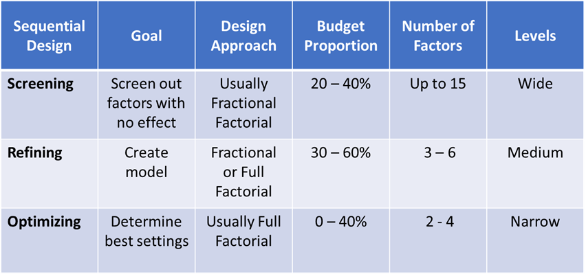
Secondly, the best strategy is to perform a series of two to three smaller experiments, rather than one large experiment. This approach is known as Sequential Designed Experiments. The first experiment is referred to as a Screening DOE. The goal is to sort out the factors (input variables) which have an effect on the output variables. And eliminate those which have no effect. The second experiment is called a Refining DOE. The goal here is to develop a mathematical model to explain the relationship between inputs and outputs. In some situations, a third experiment is run, an Optimizing DOE. The goal is to determine the best settings of inputs to achieve a specific goal of the output.
Comparison of Designed Experiments
Before going any farther, it is important to mention the Prerequisites to Successful Experimental Design. First, make sure the measurement system is adequate for the response. This should be done by performing Measurement System Analysis (MSA). If the measurement system is inadequate it must be fixed. Secondly, confirm the process is in statistical control. If the process is not in control, an experiment might indicate there was an effect due to changes to an input when in reality the effect was due to special cause variation.
Now, here is a checklist of the activities for a successful Designed Experiment:
- Plan DOE, and agree on purpose of the study
- Select response variable(s) to be studied
- Choose factors and levels
- Determine feasible number of experimental runs
- Consider blocking, interaction, center points, etc.
- Determine design and check power. Adjust design, if needed.
- Determine data collection plan
- Run experiment and collect data
- Analyze data, develop model, check residuals
- Perform confirmation run
- Prepare conclusions and write report
Screening DOEs, mentioned above, are typically done using a Fractional Factorial design. This approach will run a fraction of the total number of experimental runs for a Full Factorial Experiment. If we run half of the total experimental runs, we call this a ½ factional factorial. If we run ¼ of the experimental runs, we call this a quarter fractional factorial, and so on. Running only part of the experiment requires less resources, but some factors are confounded. Confounding or aliasing means that the effect of some factors or interactions can’t be separated.
Before running actual experiments, it is imperative to perform Step 6: Check the Power of the design. Power refers to the ability of a statistical analysis to detect an effect of a given size. Higher Power is better. Inadequate Power is one of the leading causes of failed DOEs. A common goal for Power is at least 0.90 (i.e., 90%). Some practitioners might accept a little lower value, say only 80%.
Power can be calculated in Minitab using the key elements of the design:
- Number of Factors
- Number of Experimental runs in Base Design
- Number of Replicates
- Size of the Effect
- Process Standard Deviation
- Number of Center Points.
Replicates means running the entire series of experimental runs more than once. For example, if there are eight experimental runs in the base design, but two replicates, that means a total of 16 experimental runs. A special type of experimental run is a Center Point. If the input is continuous the Center Point is achieved by running the experiment with input values halfway between the maximum and minimum levels.
If Power is too low for a design how can it be increased?
Here are the options for increasing Power:
- Decrease number of Factors
- Increase number of Runs in Base Design
- Increase number of Replicates
- Increase size of the Effect
- Decrease process Standard Deviation
- Increase number of Center Points
As you can see, there are many decisions to make when designing an experiment. Therefore, planning is so important and can take so much time. Fortunately, Minitab makes it easy to try different combinations of Replicates, Center Points, etc.
Now, to the story of the Black Belt we were coaching. Last month the BB decided to conduct a designed experiment where the response was the density of glass fiber used in making insulation. The BB worked with his team to identify six factors for the experiment. They then chose low and high levels for each factor that were as broad as possible. The team also confirmed all experimental runs (i.e., all possible combinations of factors and levels) were feasible.
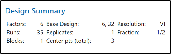
After extensive planning and discussion, the belt chose a designed experiment that was a half-fractional factorial, with 6 factors, 3 center points and 2 repeats. A Repeat is performed when more than one data value is collected for a specific experimental setup. To be clear, his initial design did not have adequate Power. Because it was too low, we thought 2 replicates might be necessary. However, that would have resulted in 64 experimental runs. He knew the project sponsor would never approve that. The BB decided to check the Power with 3 center points. This design resulted in a power of 0.907, which is very good. This allowed the belt to go forward with a design with only 35 experimental runs, instead of 64 as first planned. Scroll to the bottom of this blog to see the design for this experiment. Note the inputs are shown with Xs, and the output (response) with a Y. Also, the experimental runs (StdOrder or Standard Order) are randomized, which is a best practice with DOE.
Here is the Base Design from Minitab:
For each experimental run the project team collected response data twice. In other words, there were 2 repeats. The BB calculated the average of these two values and used this as the response. If the values were higher than 5% different, a third run was conducted to determine if it was an outlier.
Before running the experiment, the project team gathered 27 data points of historical data as a baseline. The Black Belt used Minitab to check for outliers, and to confirm if data was normally distributed, and if the process was stable and in control. The good news: There were no outliers, the process was normally distributed, and – best of all – it was in control. He also checked process capability. A Ppk = 1, which is a decent value.
The BB’s team ran the 35 experimental runs and collected response data for each one. Again, these runs were conducted in random order.
Now the BB was ready to analyze the results of the experiment. During a coaching session we suggested that he only consider 2-way interactions. After reducing the model, the belt ended up including all 6 factors but only one 2-way interaction was statistically significant.
Next, the belt checked the residual plots. He noticed one experimental run was extremely unusual. After checking the data, the BB determined there was a data entry error for this run. After correcting this mistake and re-analyzing the results the belt determined there were no unusual observations and the model had an adjusted R2 = 95.6, which is really good.
Finally, the belt used the Response Optimizer to determine the setting for each factor to achieve a specific density target. The next step, which is still pending, is to perform a confirmation run. The Black Belt plans to run the process with the settings from the Optimizer to compare the actual process output – the glass fiber density – against the predicted fiber density from the Optimizer. If the agreement between the output from Response Optimizer and the actual results is within 4%, we will conclude that the model is validated. We may validate the model at different settings. The financial impact of this project is expected to be over several million dollars.
If you’ve never run a DOE, you should seek the input from an experienced Black Belt or Master Black Belt. Do not hesitate to contact TMAC for assistance.
Good luck in your next DOE.

