
Design of Experiments: A Case Study – Part 1
Co-Authored by Alberto Yáñez-Moreno, Ph.D and Russ Aikman, MBB
Recently TMAC was providing coaching for a Black Belt working in the Analyze Phase of his project. He was trying to figure out how to increase the output for a manufacturing process. The company was in a sold-out position – demand exceeded supply. The process was production of glass fibers used in the manufacture of different types of insulation. The manufacture of glass fibers is a highly complex process. The BB determined additional capacity could result in a sales increase of over $1M. Past efforts in determining root cause of the capacity issue had been only partly successful. After discussion with the belt and his sponsor a decision was made to use Design of Experiments (DOE).
Before going into detail about this particular project, let’s start with some fundamental questions:
- What is a Designed Experiment?
- When is DOE recommended?
- What other root cause tools might be used?
- What are the pros and cons of DOE compared to other tools?
To answer these questions, we should begin with a review of Analyze Phase concepts. All LSS practitioners are familiar with the equation: Y = f(X1, X2, X3,…), where the “Y” is the process output or response variable. It is also called the Key Process Output Variable (KPOV) or the dependent variable. In terms of LSS, the “Y” is related to what we want to predict or how are we going to measure the success of the project. The “Xs” represent process inputs, and may also be called factors, Key Process Input Variables (KPIVs), or independent variables. The “f” is simply the function or formula that would allow us to predict the “Y”.
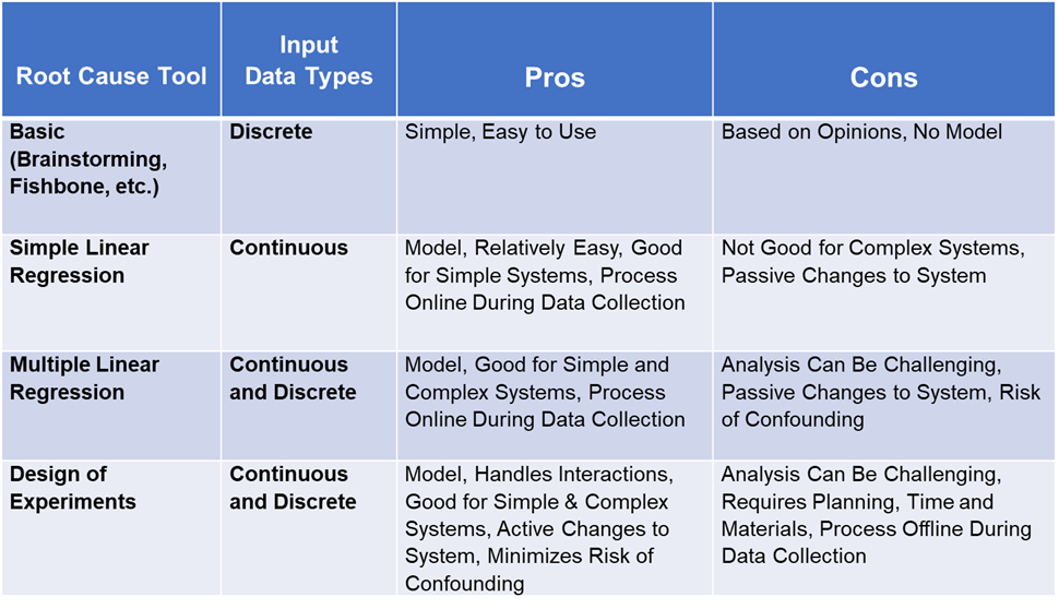
Before considering DOE, always start with more basic tools. If you have no hard data, then you can try tools like brainstorming, fishbone diagram, or C&E matrix. Such tools are always acceptable in the early stages of root cause analysis. They are simple and easy to use. And for less complex problems basic root cause tools work just fine.
But for more complex problems there is a big downside to these tools: We do not get a mathematical model. Another downside: Basic root cause tools are very dependent on process knowledge. And hence, are subject to people’s opinions. Still, basic root cause tools can be very helpful in determining what input variables to consider for more advanced tools like DOE.
Let’s say you do have historical X and Y data. In this case a good place to start is with either Simple or Multiple Linear Regression. Both can be used to generate mathematical models. And with powerful statistical software like Minitab development of a mathematical is relatively easy.
The limitation of Simple Regression is it only has one X in the model. Most real-world systems are much too complex to be modeled with a single input. Hence, Multiple Regression is a better option because it allows models with two or more inputs. Very sophisticated models can be developed using Multiple Regression.
What are the downsides to Multiple Regression? A big negative is that it does not identify interactions. An interaction occurs when changes to two or more inputs cause an effect on the output. To be fair, a person with deep knowledge of statistics can use regression to create a model which includes interactions. But for the typical LSS practitioner this is not easy to do.
There is another downside to all three of these tools: They are limited by the historical data available. Imagine a process where there is a big change in the Y when the X gets to a certain level. For example, an annealing process where oven temperature greatly impacts steel hardness once it gets above a certain level. You would never learn this if day to day operations limit oven temperatures to lower levels. Another example: Say there is a process involving inputs of time and pressure. If there is an interaction between these two inputs you might never learn of the interaction unless they were changed in a specific way.
Now, back to the questions at the start of this blog. First, what is Design of Experiments? DOE is a strategy for conducting scientific investigation of a process for the purpose of gaining information about the process. This is accomplished by actively changing specific inputs to determine their effect on outputs. A key thing to keep in mind: DOE will provide the most information possible using the least amount of resources. Stated differently, Designed Experiments allow you to learn more about how a process works with less data.
When is DOE a good tool to use?
This is the first key differentiator between DOE and regression: How data are collected. With regression, data are gathered as a part of normal operations. In other words, when the process is running normally output data is collected along with the regular input settings. The values for the input setting are typically chosen from standard operating procedures or product specifications.
With Designed Experiments data collection is different. First, the input values for the designed experiment are chosen so as to learn as much as possible about their effect on the process output. This means the input values chosen – known as the factor levels – are often outside the normal range of input settings. Most DOE experiments have just two levels – low and high for a continuous input. Each experimental run consists of a combination of input settings at these low and high values.
Imagine a process where the typical range for an input, say pressure, is 100 to 200 psi. For a Designed Experiment the two levels chosen might be 80 (low) and 220 (high) psi. Choosing input levels outside the regular operating range is likely to result in greater insight about how that input impacts the output.
Another differentiator with Designed Experiments is that changes in the input levels from experimental run to run are done randomly. The use of randomization is of critical importance to DOEs. By randomizing the experiment, a practitioner minimizes the risk of confounding. This occurs when there appears to be an effect due to one input when in reality it is due to a different input. Or the effect may be due to a ‘noise’ variable, such as ambient temperature or barometric pressure. Confounding can – and does – occur as part of regular, day-to-day operations. And hence can greatly complicate the use of regression as a root cause tool.
Finally, DOE is very good at separating out the effects of specific inputs and interactions. Other tools, like regression, are not as effective at achieving this goal which is important in development of a useful mathematical model.
Other advantages of Designed Experiments:
- Use a structured, planned approach
- Statistical significance of results is known
- Can be used for screening out factors (inputs) that have no effect on the response
- Can be used to determine optimal values for inputs to achieve project goals
- It can be applied in a wide variety of businesses including agriculture, manufacturing, service, marketing, social work, and medical research
Comparison of Root Cause Tools
In Part 2 we will discuss how to plan and conduct a DOE. And we’ll will share information about the experiment conducted by the Black Belt who received TMAC coaching, and the results he achieved.
