
Process Capability: A Critical Management Tool (Part 3)
In the previous blogs we covered the basics of process capability and its use as a Management tool. Part 1 addressed process capability for continuous, normally distributed data. Part 2 covered Short Term vs. Long Term capability, plus capability analysis when the target is not centered between the spec limits. You can read those blogs by clicking on these links:
Process Capability: A Critical Management Tool – Part 1
Process Capability: A Critical Management Tool – Part 2
In this third installment in our series we will discuss capability with continuous, non-normal data.
First – a quick review on the prerequisites to performing capability analysis, as stated in Part 1 of this blog:
- What is the business question? [How does process performance impact business goals?]
- What are the process requirements (VOC)? [What are the specifications?]
- Are process data available (VOP)? [Is there enough data, in the proper format, to characterize the process? Is the data representative of the process?]
- Can you trust the data? [Is the measurement system used to collect the data adequate?]
- Is the underlying process under control? [Is the process consistent and stable enough to trust the capability results?]
- Finally, are the data normally distributed? Or some other distribution? [While data distribution is not a limitation to performing capability analysis, knowing this is critical to ensure the right statistical analysis is performed.]
Let’s assume you met the prerequisites for items 1 to 5. Now you must determine the distribution. First – how to answer the question of whether the process is normally distributed? This can be done in Minitab by using a Graphical Summary or Probability Plot. For both of these analyses a hypothesis test is performed in which the null hypothesis assumes that the process data are normal, and the alternative is the data are from some other distribution. Like all hypothesis tests it generates a p-value. If the p value is low (less than alpha) the null is rejected (that means data are not normal) and if it is high the null is confirmed (data are normal).
A common question: What types of processes generate data that aren’t normally distributed? Examples include process lead time, contamination levels, and machine efficiency.
Determining The Distribution
Step 6 in the capability checklist is to determine the distribution. Most statistical software packages have a feature to do that including Minitab where it is called Individual Distribution Identification (available on the Stats>Quality Tools submenu). Let’s look at an example to show how this works.
Imagine a LSS team is working to improve the process lead time to sort paperwork received daily at a large insurance company. Basically, batches of insurance claims arrive by mail each day. Here is what the data looks like using the graphical summary:
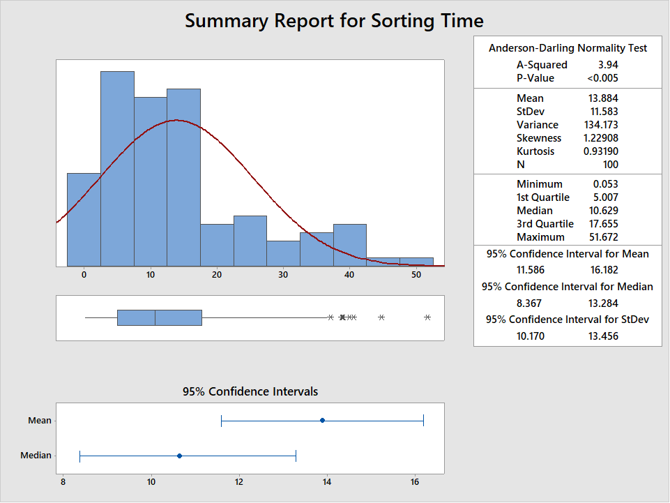
Clearly the data aren’t normally distributed, with a p-value < .05. The data is collected in subgroups of 4. We confirm that the process is in control using an Xbar-R Chart:
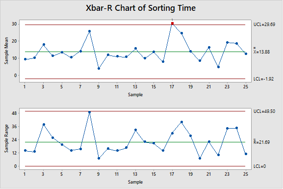
There is one data point outside the UCL for the X-Bar chart. This out of control point should be investigated. However, for practical purposes we will consider this process to be in control.
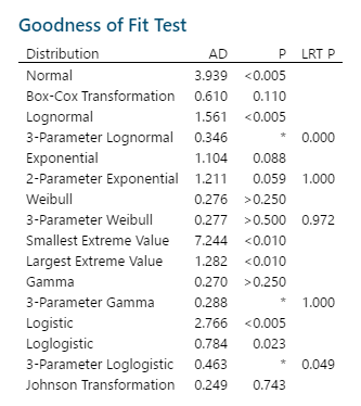
Now, let’s use the Individual Distribution Identification tool. Here is the most important output:
How to determine the distribution that best fits the data? Here are some guidelines:
- Keep in mind: Only one distribution may fit. Or multiple distributions may fit. Or none may fit. If none fit, that could be due to either (a) process is out of control or (b) sample data contains a mix of data from different processes. Other issues could also cause this problem.
- In general, the higher the p-value the better the fit. Preferably the p-value is 0.1 or higher. But it must be at least 0.05.
- If the p-value is high for multiple distributions, choose the one with the lowest AD (Anderson-Darling statistic).
- Some distributions have a basic version and a
more complex version (e.g., Lognormal and 3-Parameter Lognormal). To decide
which is best-fitting use the LRT P (Likelihood Ratio Test p-value):
- LRT P < .05 – use the more complicated version
- LRT P >= .05 – use the simpler version
- Ignore transformations. There are more negatives than positives with them in LSS applications.
Back to the Individual Distribution Identification output. For this scenario any of these distributions will work: Exponential, Weibull, or Gamma. Note that while the 3-Parameter Weibull has the highest p-value (0.5) it also has a high LRT p (0.972) indicating the basic Weibull is better for this data set.
The ‘best fitting’ appears to be Gamma, given that it has a p-value as high (or higher) than the others and the lowest AD. But as stated above any of the three distributions will work just fine.
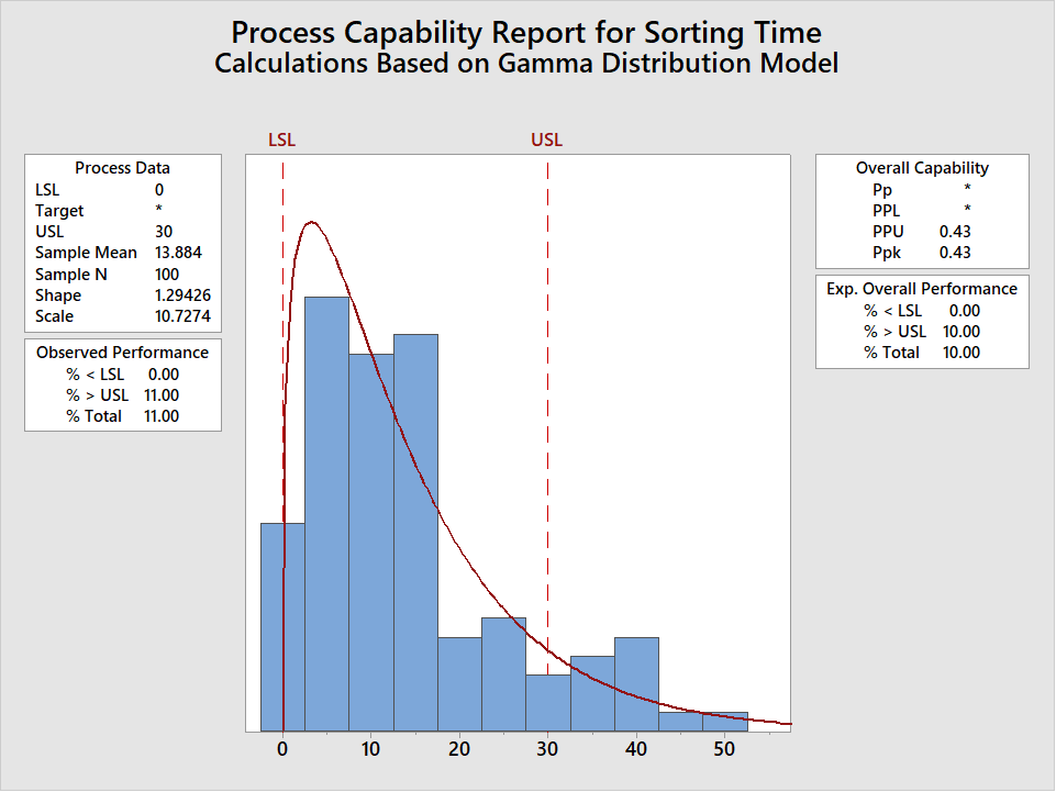
Calculating Non-Normal Capability
Now that the distribution has been determined the Non-Normal Capability Analysis can be calculated (In Minitab at Stats>Quality Tools>Capability>Non-Normal). Actually, the recommended approach is to calculate the Capability for each distribution that fits then to report the lowest value for Ppk. This is the most conservative approach. For this example the resulting Ppk is 0.43, using the Gamma Distribution, and based on a Lower Spec Limit = 0 and an Upper Spec Limit = 30 minutes.
Note that Minitab generates a Pp and Ppk, but not a Cp and Cpk. The Cp and Cpk values are not generated because they are based on a symmetric distribution (i.e., normal distribution). Because non-normal distributions are not symmetric we use different formulas to calculate the Pp and Ppk values:
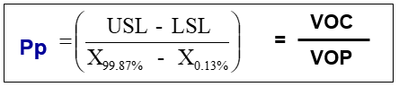

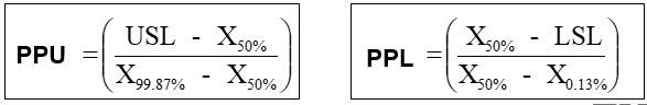
This range of values – between 99.87 and 0.13 percentiles – is equivalent to the spread of values for the normal distribution of +/- 3 standard deviations. And the median – the value of X at the midpoint (50%) of the sample – is used in place of the mean.
Regardless of the formulas used and the distribution, if the prerequisites of process capability have been met it is important to calculate the appropriate capability index. This value can be used to establish the baseline of a process, to determine the level of improvement achieved during a pilot of a solution, or to document long-term process performance.
